Maximum Likelihood Estimation in R

Suppose we want to estimate the parameters of the following AR(1) process: $$z_t=\mu +\rho (z_{t-1}-\mu )+\sigma {\epsilon }_t$$ where ${\epsilon }_t\sim N(0,1)$. We will first simulate data from the model using a particular set of parameter values. We will the write the log likelihood function of the model. Finally, the simulated dataset will be used to estimate the parameters via maximum likelihood.

Throughout this example we build an R script which can be used to replicate the experiment. First we must load the stats library which allows us to generate pseudo-random numbers from the standard Normal distribution. Second, in order to obtain reproducible results, we set the seed of the random number generator to 100:1

library('stats')
set.seed(100)

The true parameter values we use are: $\mu =-0.5$, $\rho =0.9$, and $\sigma =1$:

# True parameters
mu <- -0.5
rho <- 0.9
sigma <- 1.0

We will simulate a total of T = 10000 periods:

# Number of periods
T <- 10000

# Initialize a vector for storing the simulated data
z <- double(T)

First, we must draw an initial value of $z_1$. We use the unconditional distribution $N(\mu ,{\sigma }^2/(1-{\rho }^2))$:

# Initial draw from the unconditional distribution
z[1] <- rnorm(1, mean = mu, sd = sigma / sqrt(1 - rho^2))

Next, we simulate periods $t=2,\dots ,T$ using a for loop to take draws from the conditional distribution:

# Simulate periods t = 2..T
for (t in 2:T) {
  z[t] <- rnorm(1, mean = mu + rho*(z[t-1] - mu), sd = sigma)
}

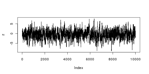
We can check to see whether the sample behaves as expected by plotting the series:

# Plot the data
png(filename = "z.png", width = 500, height = 250)
plot(z, type='l')
dev.off()

We can also compare the mean and standard deviation of the unconditional distribution with that of the sample:

# Verify the mean and standard deviation
cat('Unconditional mean:', mu, '\n')
cat('Sample mean:', mean(z), '\n')
cat('Unconditional sd:', sigma/sqrt(1 - rho^2), '\n')
cat('Sample sd:', sd(z), '\n')

This should produce something like the following:

Unconditional mean: -0.5
Sample mean: -0.5874701
Unconditional sd: 2.294157
Sample sd: 2.26217

Those value seem reasonable so we continue by writing the log likelihood function. The R function dnorm implements the density function of the Normal distribution. Thus, we simply need to sum the logged density values of $z_t$ given $z_{t-1}$ for $t=2,\dots ,T$. The log-likelihood function depends on the parameter vector $\theta$ as well as the simulated data. We write the negative log likelihood function because R wants a function which should be minimized:

# (Negative) log-likelihood function
logl <- function(theta, data) {
  T <- length(data)
  sum(-dnorm(data[2:T],
            mean = theta[1] + theta[2] * (data[1:T-1] - theta[1]),
            sd = theta[3], log = TRUE))
}

Now, with the log likelihood function in hand, we can call the nlm function to estimate $\theta$ given a starting value.

# Estimate theta
theta.start <- c(0.1, 0.1, 0.1)
out <- nlm(logl, theta.start, data = z)

The results are stored in out which contains several objects of interest such as the estimate itself, the value of the objective function, the number of iterations, etc. The results can then be reported as follows:

# Report results
cat('Estimate of theta: ', out$estimate, '\n')
cat('-2 ln L: ', 2 * out$minimum, '\n')

For the particular seed value and sample size used above, the following results were reported:

Estimate of theta:  -0.4609634 0.8911239 0.994497
-2 ln L:  28265.59