Aradillas-López and Tamer (2008)

These slides are based on the July 2007 version of the following article:

Aradillas-López, Andrés, Andres and Elie Tamer (2008). The Identification Power of Equilibrium in Games. Journal of Business and Economic Statistics 26, 261–283.

Presentation by Jason Blevins, Duke Applied Microeconometrics Reading Group, December 4, 2007.

Introduction

• Examines the identification power of Nash equilibrium assumptions.

• Compare results by dropping Nash equilibrium and using only rationalizability.

• Three examples are considered:

  • 2x2 game of complete information (e.g., Bresnahan and Reiss (1991)),

  • 2x2 game of incomplete information,

  • First price auction with independent private values.

• Given a random sample, what can we learn about a parameter of interest using only level-$k$ rationalizability.

Equilibrium Concepts

• In simultaneous-move games, players attempt to predict what their rivals will play and act accordingly.

• A Nash equilibrium occurs when players’ expectations are are consistent with their opponents’ actions.

• A Rationalizable strategy is a best response to some profile of one’s opponents’ strategies.

• Nash $\subseteq$ Rationalizable.

Behavioral assumptions

• Players use proper subjective probability distributions in analyzing uncertain events,

• Players are expected utility maximizers,

• The rules and structure of the game are common knowledge.

Rationalizability

• A strategy profile for player $i$ is dominated if there exists another strategy that is better regardless of what other players do.

• Given a profile of strategies of player $i$’s opponents, $s^{-i}$, a strategy $s^i$ for player $i$ is a best response if it is better than any other strategy given $s^{-i}$.

• Let $S^i(0)$ denote the set of player $i$’s strategies.

• We say $s^i\in S^i(0)$ is a level–1 rational strategy for player $i$ if $\exists s^{-i}\in S^{-i}(0)$ such that $s^i$ is a best response. Let $S^i(1)$ denote the set of such strategies.

• We say $s^i\in S^i(1)$ is a level–2 rational strategy for player $i$ if $\exists s^{-i}\in S^{-i}(1)$ such that $s^i$ is a best response.

• And so on…

I. 2x2 Game of Complete Information

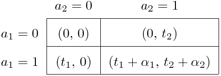
• Standard 2x2 normal-form game.

• Given a sample $\{y_{i1},y_{i2}{\}}_{i=1}^N$ of market structures (entry decisions) in $N$ independent markets.

• We want to learn about the joint distribution of $(t_1,t_2)$ as well as the parameters ${\alpha }_1$ and ${\alpha }_2$.

• Assume that ${\alpha }_1,{\alpha }_2\le 0$.

I. Level–1 rationality

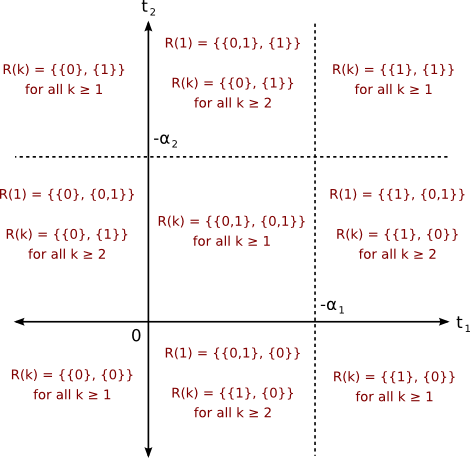
• If $t_1+{\alpha }_1\ge 0$, then $a_1=1$ is a dominant strategy for player 1.

• If $t_1<0$, $a_1=0$, then is a dominant strategy.

• If $t_1+{\alpha }_1\le 0\le t_1$, then both $a_1=0$ and $a_1=0$ are level–1 rational. They are best responses, respectively, when player 2 plays 1 or 0.

• Similarly for player 2.

I. Level–1 Rationality: Predictions

• In the middle region on the right side, note that player 2 does not rationally consider that player 1 would never play 0 in level–1 rationality. This illustrates the sequential nature of rationality.

I. Level–2 rationality

• Consider the region $(t_1,t_2)\in [-{\alpha }_1,\mathrm{\infty })\times [0,-{\alpha }_2]$.

• $ℛ(1)=\{\{1\},\{0,1\}\}$

• Player 2 believes player 1 will play $a_1=1$ with probability 1.

• $a_2=0$ is a best response.

• We can eliminate $a_2=1$ at level 2.

• $ℛ(k)=\{\{1\},\{0\}\}$ for $k\ge 2$.

I. Inference

• Suppose we know the outcome probabilities $P(0,0),\dots ,P(1,1)$.
• Object of interest: $\theta =({\alpha }_1,{\alpha }_2,F(\cdot ,\cdot ))$.
• $F(\cdot ,\cdot )$ is the joint distribution of $(t_1,t_2)$.
• Level–1 rationality implies the following restrictions on $\theta$:

$$\begin{array}{rl}\mathrm{Pr}(t_1\ge -{\alpha }_1,t_2\ge -{\alpha }_2)& \le P(1,1)\le \mathrm{Pr}(t_1\ge 0,t_2\ge 0)\\ \mathrm{Pr}(t_1\le 0,t_2\le 0)& \le P(0,0)\le \mathrm{Pr}(t_1\le -{\alpha }_1,t_2\le {\alpha }_2)\\ \mathrm{Pr}(t_1\ge -{\alpha }_1,t_2\le 0)& \le P(1,0)\le \mathrm{Pr}(t_1\ge 0,t_2\le -{\alpha }_2)\\ \mathrm{Pr}(t_1\le 0,t_2\ge -{\alpha }_2)& \le P(0,1)\le \mathrm{Pr}(t_1\le -{\alpha }_1,t_2\ge 0)\\ \end{array}$$

• The identified set ${\Theta }_I$ is the set of all $\theta$ which satisfy these inequalities.
• The model point identifies $\theta$ if ${\Theta }_I$ is a singleton.

II. 2x2 Game of Incomplete Information

• Now assume that $t_1$ and $t_2$ are private information.

• Common prior assumption on the joint distribution of $(t_1,t_2)$.

• Players have beliefs about their opponents’ actions, conditional on their own type: ${\mathbb{P}}_{t_1}\equiv \mathrm{Pr}(a_2=1|t_1).$

• As before, assume that ${\alpha }_p\le 0$ for $p=1,2$.

• The expected payoffs are now: $$U(a_i,P_{t_i})=\{\begin{array}{ll}{t}_i+{\alpha }_i{\mathbb{P}}_{t_i}& \text{if}{a}_i=1\\ 0& \text{otherwise}\\ \end{array}$$

II. Rationality

• Consider only threshold strategies: $Y_p=1\{t_p\ge {\mu }_p\}$ for $p=1,2$.

• Beliefs are thus probability distributions for ${\mu }_{-p}$ given ${ℐ}_p$ (which includes $t_p$): ${\hat{G}}_p({\mu }_{-p}|{ℐ}_p).$ This assumption effectively reduces the space of possible strategies to $ℝ$.

• The concept of rationality now has to account for level-$k$ rational beliefs. Beliefs are not required to be “correct.” Compare this with BNE beliefs, where all players know them to be correct.

• Level-$k$ rationalizable beliefs ${\hat{G}}_p({\mu }_{-p}|{ℐ}_p)$ assign zero probability to strictly dominated strategies by player $-p$.

• A strategy by player $p$ is level-$k$ rationalizable if it is a best response given level-$k$ rationalizable beliefs:

$$Y_p=1\{t_p+{\alpha }_p{\int }_{𝕊({\hat{G}}_p)}E[1\{t_{-p}\ge \mu \}|{ℐ}_p,\mu ]d{\hat{G}}_p(\mu |{ℐ}_p)\ge 0\}$$

• The support $𝕊({\hat{G}}_p)$ of by applying iterated elimination of dominated strategies.

II. Level–1 rationality

• For any belief function, the following must hold eventwise: $$1\{t_p+{\alpha }_p\ge 0\}\le 1\{Y_p=1\}\text{and}1\{t_p<0\}\le 1\{Y_p=0\}$$

• All other decision rules are strictly dominated for all possible beliefs.

• The above inequalities imply $$\mathrm{Pr}(t_p+{\alpha }_p\ge 0)\le \mathrm{Pr}(t_p\ge {\mu }_p)\le \mathrm{Pr}(t_p\ge 0)$$ or simply, ${\mu }_p\in [0,-{\alpha }_p]$.

• This is the set of level–1 rationalizable strategies.

II. Level–2 rationality

• Level 2 rationalizable beliefs:

  • assign zero probability to strictly dominated strategies ${\mu }_p\notin [0,-{\alpha }_p]$,

  • satisfy $\hat{G}(0|{ℐ}_p)=0$ and $\hat{G}(-{\alpha }_p|{ℐ}_p)=1$.

• Level 2 rationalizable strategies are:

  • level 1 rationalizable (i.e., $0\le {\mu }_p\le -{\alpha }_p$),

  • best responses given level–2 rational beliefs.

• A strategy $Y_p=1\{t_p\ge {\mu }_p\}$ is level–2 rationalizable if $${\mu }_p=-{\alpha }_p{\int }_0^{-{\alpha }_{-p}}E[1\{t_{-p}\ge \mu \}|{ℐ}_p,\mu ]d{\hat{G}}_p(\mu |{ℐ}_p)$$

II. Level-k rationality

We can summarize the set of level-$k$ rationalizable strategies in the class of threshold strategies $Y_p=1\{t_p\ge {\mu }_p\}$ as follows:

• For $k=1$ and $p\in \{1,2\}$, $${\mu }_p\in [{\mu }_{p,k}^L,{\mu }_{p,k}^U]\equiv [0,-{\alpha }_p]$$

• For $k>1$ and $p\in \{1,2\}$, $${\mu }_p\in [{\mu }_{p,k}^L,{\mu }_{p,k}^U]\equiv [-{\alpha }_{p}E[1\{t_{-p}\ge {\mu }_{-p,k-1}^U\}|{ℐ}_p],-{\alpha }_{p}E[1\{t_{-p}\ge {\mu }_{-p,k-1}^L\}|{ℐ}_p]]$$

• Note that $[{\mu }_{p,k}^L,{\mu }_{p,k}^U]\subseteq [{\mu }_{p,k-1}^L,{\mu }_{p,k-1}^U]$ for any $k>1$ a.s.

• Any level-$k$ rational player is also level-$k\prime$ rational for any $1\le k\prime \le k-1$.

• If there is a unique BNE $({\mu }_1^{\star },{\mu }_2^{\star })$, then $$\underset{k\to \mathrm{\infty }}{\lim }[{\mu }_{p,k}^L,{\mu }_{p,k}^U]=\{{\mu }_p^{\star }\}.$$

II. A Parametric Model

• Let $t_p=X_p^{\top }{\beta }_p-{\epsilon }_p$ for $p\in \{1,2\}$ where $X_p$ is observable to the researcher but ${\epsilon }_p$ is not. We wish to estimate ${\beta }_p$.

• For simplicity, ${\epsilon }_1$ and ${\epsilon }_2$ are independent and ${\epsilon }_p\sim H_p(\cdot )$.

• Player $p$ knows ${\epsilon }_p$ and believes ${\epsilon }_{-p}\sim H_{-p}(\cdot )$.

• We now proceeds as follows:

  1. Develop an objective function which can be used to construct the identified set ${\Theta }_I$,

  2. Discuss identification of $k$,

  3. Provide sufficient conditions for point identification.

II. Iterative Construction of Beliefs

• We no longer restrict ourselves to threshold strategies.

• Let $ℐ$ be the information set of both players as well as the econometrician (i.e., the regressors).

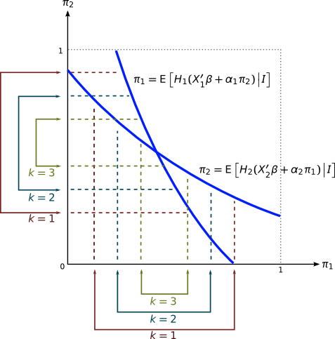
• We iteratively construct bounds on the beliefs $\mathrm{Pr}(Y_{-p}|ℐ)$: $${\pi }_{-p}^L(\theta |k,ℐ)\le \mathrm{Pr}(Y_{-p}|ℐ)\le {\pi }_{-p}^U(\theta |k,ℐ).$$

• Initialize ${\pi }_{-p}^L(\theta |k=1,ℐ)=0$ and ${\pi }_{-p}^U(\theta |k=1,ℐ)=1$.

• Then for each $k>1$ and each $p\in \{1,2\}$: $$\begin{array}{c}{\pi }_p^L(\theta |k,ℐ)=H_p(X_p^{\top }{\beta }_p+{\alpha }_p{\pi }_{-p}^U(\theta |k-1,ℐ)),\\ {\pi }_p^U(\theta |k,ℐ)=H_p(X_p^{\top }{\beta }_p+{\alpha }_p{\pi }_{-p}^L(\theta |k-1,ℐ)).\end{array}$$

• It follows that $$[{\pi }_{-p}^L(\theta |k,ℐ),{\pi }_{-p}^U(\theta |k,ℐ)]\subseteq [{\pi }_{-p}^L(\theta |k-1,ℐ),{\pi }_{-p}^U(\theta |k-1,ℐ)]\text{a.s.}$$

II. Iterative Belief Construction Example

II. Finding the Identified Set

• Player $p$ is $k$-rational if and only if $$1\{X_p^{\top }{\beta }_p+{\alpha }_p{\pi }_{-p}^U(\theta |k,ℐ)\ge {\epsilon }_p\}\le 1\{Y_p=1\}\le 1\{X_p^{\top }{\beta }_p+{\alpha }_p{\pi }_{-p}^L(\theta |k,ℐ)\ge {\epsilon }_p\}$$

• We can use this relationship as a basis for inference.

• Given some $k$, let $W_p\equiv (X_p,ℐ)$ and let $a,b\in {ℝ}^{dim(W_p)}$: $${\Lambda }_p(\theta |a,b,k)=E\left[(1-1\left\{\begin{array}{c}{H}_p(X_p^{\top }{\beta }_p+{\alpha }_p{\pi }_{-p}^U(\theta |k,ℐ))\\ \le \mathrm{Pr}(Y_p=1|W_p)\\ \le H_p(X_p^{\top }{\beta }_p+{\alpha }_p{\pi }_{-p}^L(\theta |k,ℐ))\end{array}\right\})1\{a\le W_p\le b\}\right].$$

• Then define $${\Gamma }_p(\theta |k)=\iint {\Lambda }_p(\theta |a,b,k){\mathrm{dF}}_{W_p}(a){\mathrm{dF}}_{W_p}(b)\text{and}\Gamma (\theta |k)={({\Gamma }_1(\theta |k),{\Gamma }_2(\theta |k))}^{\top }$$

II. Finding the Identified Set

• We can use the previous expression to construct an objective function.

• For some positive definite matrix $\Omega$, $$\Theta (k)=\{\theta \in \arg \underset{\theta }{\min }Q(\theta |k)\equiv \arg \underset{\theta }{\min }\Gamma (\theta |k{)}^{\top }\Omega \Gamma (\theta |k)\}.$$

• By construction, $\Theta (k+1)\subseteq \Theta (k)$ for all $k$.

• Given a random sample, we can use set inference methods to construct an estimator for $\Theta (k)$.

• As compared with Nash equilibrium, we do not have to solve a fixed point problem. The iterative restrictions imposed by rationality are computationally simple by comparison.

• For any $k$, $\Theta (k)$ is guaranteed to contain the BNE.

II. Inference on the Rationality Level

• A sample can also inform us about the level of rationality $k$.

• Suppose all players are at most $k_0$-rational.

• The level-$k_0$ bounds should hold a.e. but the level-$(k_0+1)$ bounds may be violated.

• We can proceed as follows:

  • Construct $\Theta (1)$,

  • Define $\tilde{Q}(k)={\min }_{\theta \in \Theta (1)}Q(\theta |k)$,

  • $\tilde{Q}(k)=0$ for $k\le k_0$ but $\tilde{Q}(k)>0$ if $k>k_0$.

• Thus, if $\tilde{Q}(k)>0$ and $\tilde{Q}(k-1)=0$ we can reject $k_0=k$.

II. Point Identification Under Level–1 Rationality

• Suppose players are level–1 rational.

• Suppose $X_p$ has full rank for $p\in \{1,2\}$. Let $X_{d,p}$ and $X_{l,p}$ denote, respectively, regressors with bounded and unbounded support and let ${\beta }_{d,p}$ and ${\beta }_{l,p}$ be the corresponding coefficients. Finally, define $X\equiv (X_1,X_2)$.

• ${\beta }_{l,p}$ is identified if for each $p$, there is a continuous $X_{l,p}$ with nonzero ${\beta }_{l,p}$ and unbounded support conditional on $X_{-l,p}$ such that for any $c\in (0,1)$, $b\ne 0$ and $q\in {ℝ}^{dim(X_{-l,p})}$, there exists $C_{b,q,m}>0$ such that $$\mathrm{Pr}({\epsilon }_p\le b{X}_{l,p}+q^{\top }{X}_{-l,p}|X)>m$$ for all $X_{l,p}$ and $sgn(b)\cdot X_{l,p}>C_{b,q,m}$.

II. Point Identification Under Level–1 Rationality

• ${\beta }_{d,p}$ is identified if for any ${\alpha }_p,{\beta }_{d,p},{\tilde{\beta }}_{d,p}\in \Theta$ with ${\tilde{\beta }}_{d,p}\ne {\beta }_{d,p}$, $$\mathrm{Pr}(|X_{d,p}^{\top }({\beta }_{d,p}-{\tilde{\beta }}_{d,p})|>\left|{\alpha }_p\right||X_{-d,p})>0.$$

• If the above two properties hold, and for any $\Delta >0$, there exists ${𝒳}_{\Delta }\in 𝕊(X_p)$ such that $\mathrm{Pr}(Y_p=1|X)<\mathrm{Pr}({\epsilon }_p\le X_p^{\top }{\beta }_{b_0}+{\alpha }_{p_0}|X)+\Delta$ whenever $X_p\in {𝒳}_{\Delta }$, then the identified set for ${\alpha }_p$ is $\{{\alpha }_p\le {\alpha }_{p_0}\}$.

III. First Price IPV Auction

• Many symmetric, risk-neutral potential buyers.

• Bids are made simultaneously for a single good.

• Focus on independent private values (IPV) $v_i$.

• Object of interest: $F_0(\cdot )$, the distribution of private values.

• $F_0(\cdot )$ is common knowledge among all players; has support $[0,\omega )$.

• For simplicity, assume the reserve price is $p_0=0$.

III. Interim Rationality

• Point identification in BNE case established by Guerre, Perrigne and Vuong (2000).

• Here, the equilibrium assumption is relaxed following Battigalli and Siniscalchi (2003).

• Buyers under interim rationality:

  • rational,

  • expected utility maximizers,

  • strategically sophisticated to a particular degree $k$,

  • have beliefs that may or may not be “correct.”

III. Assumptions on Beliefs

• Bidders expect that any positive bid will win with positive probability:

  • No player will bid higher than $v_i$,

  • Each bidder with $v_i>0$ will submit a strictly positive bid.

  • The number of potential bidders $𝒩$ equals the number of actual bidders a.s.

• Beliefs only assign positive probability to increasing bidding functions.

• The space of all such functions is $$ℬ=\{b(\cdot ):[0,\omega )\to {ℝ}_{+}|b(v)\le v\text{and}v>w\Rightarrow b(v)>b(w)\}.$$

III. Level–1 Rationality

• Player $i$’s problem is $$\underset{b\ge 0}{\max }(v_i-b){\widehat{\mathrm{Pr}}}_i[\underset{j\ne i}{\max }b(v_j)\le b].$$

• Here, ${\widehat{\mathrm{Pr}}}_i$ denotes player $i$’s beliefs about $v_{-i}$.

• Level–1 rational bid satisfy $$b\le v_i\equiv {\overline{B}}_1(v_i,𝒩).$$

• Any bid show any bid below $v_i$ is level–1 rational (and thus we cannot bound bids from below).

III. Level–2 Rationality

• The worst case scenario for player $i$ is that for all $j$, $$b(v_j)={\overline{B}}_1(v_j,𝒩)=v_j.$$

• Expected utility in this case is $$\underset{b\ge 0}{\max }(v_i-b){\widehat{\mathrm{Pr}}}_i[\underset{j\ne i}{\max }{\overline{B}}_1(v_j,𝒩)\le b]=\underset{b\ge 0}{\max }(v_i-b)F_0(b{)}^{𝒩-1}\equiv {\pi }_2(v_i,𝒩).$$

• ${\pi }_2(v_i,𝒩)$ is thus a lower bound over all beliefs. The upper bound is $(v_i-b)$.

• Thus, rational bids must satisfy $$v_i-b\ge {\pi }_2(v_i,𝒩)$$ or $$b\le v_i-{\pi }_2(v_i,𝒩)\equiv {\overline{B}}_2(v_i,𝒩).$$

III. Level-k Rationality

• Proceeding recursively, one can show that at level-$k$, $$b_i\le v_i-{\pi }_k(v_i,𝒩)\equiv {\overline{B}}_k(v_i,𝒩)$$ where $${\pi }_k(v_i,𝒩)=\underset{b\ge 0}{\max }(v_i-b)F_0{({\overline{S}}_{k-1}(b,𝒩))}^{𝒩-1}$$ and $${\overline{S}}_{k-1}(b,𝒩)\equiv {\overline{B}}_k^{-1}(\cdot ,𝒩).$$

• We know that ${\overline{B}}_k(\cdot ,𝒩)\ge b^{\mathrm{BNE}}(\cdot ,𝒩)$ for all $k$. Furthermore, bidding below $b^{\mathrm{BNE}}$ is rationalizable for all $k$.

• That is, the predictive power of $k$-rationality in this model is significantly less than that of BNE.

III. Identification with Level–1 Rationality

• Suppose $F_0$ lies in the space of log-concave, absolutely continuous distribution functions on $[0,\omega )$.

• We are given a sample of $L$ auctions and want to recover $F$.

• The model predicts that level–1 rational bids satisfy $0\le b_i\le v_i$ for all $i=1,\dots ,𝒩$.

• The $b_i$’s are observed but the $v_i$’s are not, but we can still bound $F$: $$F_0(t,\theta )\equiv \mathrm{Pr}(v\le t)\le \mathrm{Pr}(b\le t)\equiv G_b(t).$$

• Empirical strategy: bound the distribution of valuations using the empirical distribution of bids.

III. Identification with Level-k Rationality

• Continue for $k>1$ using the bounds derived above.

• We can derive an objective function as before: $$\begin{array}{c}\Lambda (\theta |a,c,k)=\int (1-1\{F_b(b)\ge F({\overline{S}}_k(b,𝒩|\theta ),\theta )\})1\{a\le b\le c\}{\mathrm{dF}}_b(b)\\ \Lambda (\theta |k)=\iint \Lambda (\theta |a,c,k){\mathrm{dF}}_b(a){\mathrm{dF}}_b(c)\\ \Theta (k)=\{\theta \in \Theta :\theta \in \arg \underset{\theta \in \Theta }{\min }\Gamma (\theta |k{)}^2\}\\ \end{array}$$

Conclusion

• Look at identification power of Nash equilibrium by comparing to level-$k$ rationality.

• Derivation of identified set and corresponding objective functions for conducting inference.

• Three cases:

  • 2x2 game of complete information,

  • 2x2 game of incomplete information,

  • first price auction.