Graham, Imbens, and Ridder (2006)

These slides are based on the working paper “Complementarity and Aggregate Implications of Assortative Matching” by Bryan S. Graham, Guido W. Imbens, and Geert Ridder, May 14, 2006.

Presentation by Jason Blevins, Duke Applied Microeconometrics Reading Group, March 6, 2007.

Basic Model

• Reallocation of an indivisible input across firms.

• Aggregate stock of input is fixed.

• Firm output may be monotone, but at different rates.

• Cannot simultaneously increase input level for all firms.

Reallocations

• What is the effect on average output of input reallocations?

• Marginal distribution of reallocated input remains unchanged.

• Average output may change if production technology is nonseparable.

Examples

• Teacher reallocation across classrooms of varying mean student ability.

• Assignment mechanisms for college roommates in the presence of social interactions.

• Effects of spousal sorting on child education.

Estimation

• Nonparametrically estimate production function, CDFs of inputs, and quantile functions.

• Average over distribution of inputs under new assignment rule.

Comparison

• Allow for continuous treatment (rather than binary or discrete).

• Assignment policies do not change the marginal distribution of the input in the population.

• In treatment effect literature, assignment of treatment is not restricted by the treatment of other units.

• Focus on redistributions under specific assignment rules, not optimal assignment rules.

Contributions

• Develop a framework for estimating outcomes under correlated matching.

• Derive an estimator for average output under correlated matching.

• Except for perfect positive and negative rank correlation, the estimator has a parametric rate of convergence.

• Derive the asymptotic properties of the estimator in all cases.

Model

• $Y_i(w)$ output associated with input level $w$ for firm $i$.

• Interested in reallocating input $W$ across firms.

• Hold marginal distribution of $W$ fixed.

• Observed firm characteristics $X\in ℝ$, $Z\in {ℝ}^K$.

Notes:

• Holding the marginal distribution of $W$ fixed is appropriate for situations where the input is indivisible (e.g., Teachers, Managers) and when the aggregate stock of the input is hard to augment.

• $X$ is a scalar because the paper focuses on rank ordered matching. There is no clear natural ordering for vector valued covariates.

Identifying Assumption

• Unconfoundedness/Exogeneity: $$Y(w)\perp W|X,Z\text{for all}w\in 𝒲\subset ℝ.$$

• Conditional on firm characteristics $(X,Z)$, the assignment of $W$ is exogenous.

• Example: $\dim (X)=\dim (Z)=0$. Then, $Y(w)\perp W$ and consequently, $E[Y(w)]=E[Y|W=w]$.

That is, the average output we would see if all firms were assigned $W=w$ equals the average output among firms that actually have $W=w$. The distribution of potential outcomes must be the same in the subpopulation of firms that were assigned $W=w$ as that in the overall population. This is the analogous assumption to that of the binary treatment effect model of Rosenbaum and Rubin (1983).

• In general, this only has to hold within $(X,Z)$ subpopulations.

Production Function

• Define the production function $$g(w,x,z)=E[Y|W=w,X=x,Z=z].$$

• $g$ denotes average output associated with input levels $(w,x,z)$.

• Under the unconfoundedness assumption, $$g(w,x,z)=E[Y(w)|X=x,Z=z].$$

Unconfoundedness implies that among firms with identical $X$ and $Z$, the (counterfactual) average output of firms if we assigned $W=w$ to all firms is equal to the actual average output of firms that are in fact assigned $W=w$.

Quantities of Interest

• Treatment effect literature has mostly looked at estimating $$E_{X,Z}[g(1,X,Z)-g(0,X,Z)].$$

• With continuous inputs, we may want to estimate $g(w,x,z)$ or $$\frac{\partial g}{\partial w}(w,x,z).$$

• This paper is concerned with policies that redistribute an input $W$ following a rule based on $X$.

• What is the average output under such a policy?

Positive Matching

• Among units with the same realization of $Z$, those with the highest values of $X$ receive the highest values of $W$.

• $${\beta }^{\text{pam}}=E\left\{g[F_{W|Z}^{-1}(F_{X|Z}(X|Z)|Z),X,Z]\right\}.$$

• $F_{X|Z}(X|Z)$ denotes the conditional CDF of $X$ given $Z$.

• $F_{W|Z}^{-1}(q|Z)$ is the quantile of order $q$ of the conditional distribution of $X$ given $Z$.

• We would expect this redistribution to perform well if there is complementarity between $X$ and $W$.

• $F_{W|Z}^{-1}(q|Z)$ is a conditional quantile function.

Graphical Example

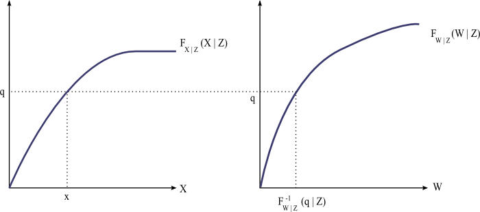
Interpretation

• Thus, $F_{W|Z}^{-1}(F_{X|Z}(X|Z)|Z)$ takes a unit’s position in the distribution of $X|Z$ and assigns to it a value of $W$ corresponding to that quantile.

• Consider instead the population-wide redistribution $${\beta }^{\text{pam2}}=E\left\{g[F_W^{-1}(F_X(X)),X,Z]\right\}.$$

• Total effect is hard to interpret: complementarity or substitutability between $W$ and $X$ is mixed with correlation between $W$ and $Z$.

• The authors focus on redistributions within subpopulations defined by $Z$ because they reflect solely the complementarity or substitutability between $W$ and $X$. Population-wide redistributions confound these effects by altering the joint distribution of $W$ and $Z$.

• However, there is a distinction to be made between what redistribution might help us learn about complementarity and which might be optimal socially.

An Example

• $W$: teacher quality.
• $X$: mean beginning-of-year achievement.
• $Z$: fraction of class that is female.
• Suppose achievement varies with gender ($X$ and $Z$ correlated).
• Positive assortative matching: high-quality teachers assigned to high-achievement classrooms.
• Alters joint distributions of $W$ and $X$ as well as $W$ and $Z$.

An Example

• This also tends to assign good teachers to classrooms with a large fraction of female students.
• Subsequent increases in achievement may reflect complementarity between $W$ and $X$.
• May also reflect how changes in teacher quality changes with gender.
• Conditional on gender, there may be no complementarity at all!
• Thus, focusing on redistributions across classrooms with similar gender mixes allows us to learn about complementarity.

Negative Matching

• $${\beta }^{\text{nam}}=E\left\{g[F_{W|Z}^{-1}(1-F_{X|Z}(X|Z)|Z),X,Z]\right\}.$$

• Example: assign best teachers to low-achievement classrooms.

Estimation

• Note that although the model was developed for $Z$ subpopulations, only population-wide estimators are presented.

• We can estimate ${\beta }^{\text{pam}}$ and ${\beta }^{\text{nam}}$ only at nonparametric rates.

• These estimators follow the analogy principle.

• Status quo: $${\beta }^{\text{sq}}=N^{-1}\sum _{i=1}^N{Y}_i$$

• For others, need $\hat{g}$, ${\hat{F}}_X$, ${\hat{F}}_W$, and ${\hat{F}}_W^{-1}$.

Estimation of g

• Nonparametric Kernel estimation of the production function $g(w,x,z)$.

• Series estimators could also be used.

• Kernel $K(u)$ with $u\in R^{K+2}$, bandwidth $b$, $V_i=(W_i,X_i,Z_i)$ and $v=(w,x,z)$.

$$\hat{g}(w,x,z)=\frac{\sum _i{Y}_{i}K\left(\frac{v-V_i}{b}\right)}{\sum _{i}K\left(\frac{v-V_i}{b}\right)}$$

Support problems: we are trying to learn about a counterfactual allocation that may involve areas of the support for which we have few observations to estimate $g$.

Estimation of CDFs

• Use empirical CDFs:

$${\hat{F}}_X(x)=N^{-1}\sum _{i}1(X_i\le x)$$ $${\hat{F}}_W(w)=N^{-1}\sum _{i}1(W_i\le w)$$

• Quantile function $F_W^{-1}(q)$:

$${\hat{F}}_W^{-1}(q)=\underset{w\in 𝒲}{\inf }1\{{\hat{F}}_W(w)\ge q\}$$

Estimation

• Estimate ${\beta }^{\text{pam}}$ and ${\beta }^{\text{nam}}$ by analogy:

$${\hat{\beta }}^{\text{pam}}=\frac{1}{N}\sum _{i=1}^N\hat{g}[{\hat{F}}_W^{-1}({\hat{F}}_X(X_i)),X_i,Z_i]$$

$${\hat{\beta }}^{\text{nam}}=\frac{1}{N}\sum _{i=1}^N\hat{g}[{\hat{F}}_W^{-1}(1-{\hat{F}}_X(X_i)),X_i,Z_i]$$

• Note that here we are averaging over both $X$ and $Z$.

• The rate of convergence of ${\hat{\beta }}^{\text{pam}}$ and ${\hat{\beta }}^{\text{nam}}$ is slower than the parametric rate.

• Loosely speaking, this is because we estimate a nonparametric function $g(w,x,z)$ with more parameters than we then average over.

Correlated Matching

• We have four focal allocations:

• Perfect positive assortative matching,

• Perfect negative assortative matching,

• The status quo,

• Random matching.

• Random matching occurs when $W$ and $X$ are independently assigned within subpopulations.

• Consider a subset of the set of all feasible allocations.

• Two-parameter subset which has the above as special cases.

• Traces paths between the four focal allocations.

Correlated Matching

• ${\beta }^{\text{cm}}(\rho ,\tau )$

• $\tau \in [0,1]$ controls nearness to the status quo (at 1).

• $\rho \in [-1,1]$ controls nearness to perfect negative or positive allocative matching.

• Focal allocations

• ${\beta }^{\text{sq}}={\beta }^{\text{cm}}(\rho ,1)$

• ${\beta }^{\text{rm}}={\beta }^{\text{cm}}(0,0)$

• ${\beta }^{\text{pam}}={\beta }^{\text{cm}}(1,0)$

• ${\beta }^{\text{nam}}={\beta }^{\text{cm}}(-1,0)$

Correlated Matching

• Status quo allocation: $${\beta }^{\text{sq}}=E[Y]=E[g(W,X,Z)].$$

• Random matching allocation: $${\beta }^{\text{rm}}=\int [\int \int g(w,z,z){\mathrm{dF}}_{W|Z}(w|z){\mathrm{dF}}_{X|Z}(x|z)]{\mathrm{dF}}_Z(z).$$

Normal Copula

• Redefine matching allocations using a truncated bivariate standard Normal copula:

$$\varphi (x_1,x_2,\rho )=\frac{1}{2\pi \sqrt{1-{\rho }^2}}\exp [-\frac{1}{2(1-{\rho }^2)}(x_1^2-2\rho x_1{x}_2+x_2^2)],$$

$${\varphi }_c(x_1,x_2,\rho )=\frac{\varphi (x_1,x_2,\rho )}{\Phi (c,c,\rho )-\Phi (c,-c,\rho )-[\Phi (-c,c,\rho )-\Phi (-c,-c,\rho )]}.$$

• The possible joint CDFs in this class are parametrized by $\rho$

$$H_{W,X}(w,x)={\Phi }_c[{\Phi }_c^{-1}(F_W(w)),{\Phi }_c^{-1}(F_X(x));\rho ].$$

Normal Copula

• Marginal CDFs: $H_{W,X}(w,\mathrm{\infty })=F_W(w)$, $H_{W,X}(\mathrm{\infty },x)=F_X(x)$.

• Special case: independent $X$ and $W$ when $\rho =0$.

• Joint PDF:

$$h_{W,X}(w,z)={\varphi }_c[{\Phi }_c^{-1}(F_W(w)),{\Phi }_c^{-1}(F_X(x));\rho ]\frac{f_W(w)f_W(x)}{{\varphi }_c\left[{\Phi }_c^{-1}(F_W(w))\right]{\varphi }_c\left[{\Phi }_c^{-1}(F_X(x))\right]}$$

Correlated Matching

• $\tau$ denotes distance from the status quo.

$$\begin{array}{rl}{\beta }^{\text{cm}}(\rho ,\tau )& =\tau E[Y]\\ & +(1-\tau )\int g(w,x,z)d\Phi ({\Phi }^{-1}(F_{W|Z}(w|z)),{\Phi }^{-1}(F_{X|Z}(x|z));\rho )F_Z(z).\end{array}$$

$${\beta }^{\text{cm}}(\rho ,0)=\int \int \int g(w,x,z)\frac{{\varphi }_c[{\Phi }_c^{-1}(F_W(w)),{\Phi }_c^{-1}(F_X(x));\rho ]}{{\varphi }_c\left[{\Phi }_c^{-1}(F_W(w))\right]{\varphi }_c\left[{\Phi }_c^{-1}(F_X(x))\right]}{f}_W(w)f_{X,Z}(x,z)\mathrm{dw}\mathrm{dx}\mathrm{dz}$$

$${\beta }^{\text{rm}}={\beta }^{\text{cm}}(0,0)=\int [\int \int g(w,z,z){\mathrm{dF}}_{W|Z}(w|z){\mathrm{dF}}_{X|Z}(x|z)]{\mathrm{dF}}_Z(z).$$

Estimation

• Analog estimator for ${\beta }^{\text{cm}}(\rho ,0)$:

$${\hat{\beta }}^{\text{cm}}(\rho ,0)=\frac{1}{N^2}\sum _{i=1}^N\sum _{j=1}^N\hat{g}(W_i,X_j,Z_j)\frac{{\varphi }_c[{\Phi }_c^{-1}({\hat{F}}_W(W_i)),{\Phi }_c^{-1}({\hat{F}}_X(X_j));\rho ]}{{\varphi }_c\left[{\Phi }_c^{-1}({\hat{F}}_W(W_i))\right]{\varphi }_c\left[{\Phi }_c^{-1}({\hat{F}}_X(X_i))\right]}$$

• Under random matching ($\rho =0$), the densities on the right hand side cancel out, leaving ${\hat{\beta }}^{\text{rm}}$.

• For $\tau >0$, we have the convex combination

$${\hat{\beta }}^{\text{cm}}(\rho ,\tau )=\tau {\hat{\beta }}^{\text{sq}}+(1-\tau ){\hat{\beta }}^{\text{cm}}(\rho ,0).$$

• This is linear in the nonparametric regression function $\hat{g}$ and nonlinear in the empirical CDFs of $X$ and $W$.

• The authors claim that under certain conditions, this estimator is consistent and asymptotically normal, but the proofs are omitted in the latest available version (May 2006).

Application

• Effects of parents’ education on education of child.

• Data: 10,272 children from the National Longitudinal Survey of Youth (NLSY).

• Simple model with three variables:

• Mother’s education

• Father’s education

• Child’s education

Summary Statistics

Regression

• Nonlinearity of the relationship suggests that education of the child might be sensitive to reallocations.

• Inspection of the data reveal that there is an asymmetry: it is better to have a mother with high education and a father with low education than vice-versa. The interaction term here doesn’t capture that.

Estimates